Summary
This post is inspired by the work of Antonio Sánchez Chinchón, and his original post on Clifford Attractors.
In a nutshell I wanted to replicate his approach whilst making three clear deviations, namely:
- using base R instead of optimised Rcpp (C++) code for the computation
- randomise the parameters to create an “infinite” number of outcomes
- save this output into many tiles
Background and Theory
Clifford attractors are infinite attractors described by 4 parameters (a, b, c, d) and 2 equations. Starting with an initial value for two values X and Y one computes the next starting point-pair. Thus the computation is sequential and this means generating point-pairs or trajectories from the previous outcome.
I chose a basic looping approach to fill a data frame of 1 million point-pairs.
The approach has several steps:
Define the global parameters (how many points to generate, how many iterations to run)
- Wrap the below steps in a loop
- Generate random parameters over a given domain using
runif - Create holder vector for the results
- Define the attractors and compute the first point
- Generate random parameters over a given domain using
Intialisation
library(scales)

# set global paramaters
xs=runif(1000000) # vector of length(~4Mb for 5x10^5)
gens=seq(1:12) # number (n) of images to generate
Main Loop
# main loop
for (j in 1:length(gens)){

# model parameters (~ 4:1 generation ratio!)
a = runif(1,min=1,max=2)*-1
b = runif(1,min=1,max=2)*-1
c = runif(1,min=1,max=2)*-1
d = runif(1,min=1,max=2)*-1

# make holder vectors
res1 <- numeric(length(xs)+1)
res2 <- numeric(length(xs)+1)

# define clifford attractors eq at X=0, Y=0
res1[1] <- sin(a)-c*cos(a)
res2[1] <- sin(b)-d*cos(b)

# sequential trajectories derived from previous values
for (i in seq_along(xs)) {
  res1[i+1] <- sin(a*res2[i])+c*cos(a*res1[i])
  res2[i+1] <- sin(b*res1[i])+d*cos(b*res2[i])
  }

}
Plot a Single Example
# single case plot
plot(res1,res2,type="p",pch=16,asp=1,
     cex=0.01,col=alpha("black",0.02),xlim=c(-3,3),
     ylim=c(-3,3),axes=FALSE,xlab="",ylab="")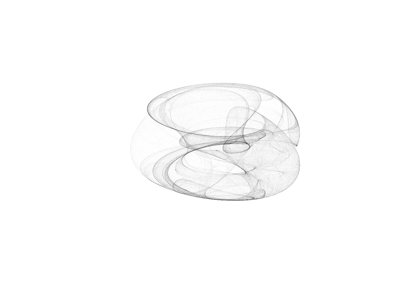
Iterate N Times as Desired
Substitute and replace the single case plot call above with this code block to generate, and save n number of iterations.
# generate distinct labels for output
lab <- paste0(sample(letters,5),collapse="")

# multiple case plotting
png(paste0("imgs/",lab,".png"),units="px", width=2000, height=2000,res=300)
plot(res1,res2,type="p",pch=16,asp=1,
     cex=0.01,col=alpha("black",0.02),xlim=c(-3,3),
     ylim=c(-3,3),axes=FALSE,xlab="",ylab="")
dev.off()