Wind and Waves in Cape Town: Part 2

Preparation of the Raw Data Files

Using the downloaded gz we can quickly get access to the data.

for i in *.gz;
do gunzip "$i";
done

Note: The downloaded files are not complete in their coverage (not all time periods) - which is something to be expected from remote/aggregated data archives.

I used the isdparser library which parses the rather esoteric .txt files. This is a slow process and took about 5 minutes for <100 files!

I therefore save the aggregated data.frame as a .txt file for later use.

# load required libraries
library(isdparser)
library(tidyverse)

# set directory of data files
filenames <- list.files()

ldf <- lapply(filenames,isd_parse,parallel=TRUE) %>% 
  lapply(.,"[",c(2,4:5,7:8,10,13:14,15,16:17,22,26)) %>% 
  dplyr::bind_rows(.)

# write data to convenient file for later quick import
write.table(ldf,file="station_tables.tsv",sep="\t",
            col.names=T,row.names = FALSE)

rm(ldf)

Initial Cleaning

A key part of the analysis is taking the incoming data and appropriately formatting it for further use by;

setting up a datetime framework
selecting variables of interest
renaming + setting appropriate data-types (chr, factor, numeric etc.)

# load extra libraries
library(tidyverse)
library(lubridate) 
library(stringr)
library(extrafont)

setwd("C:/Users/daniel/Desktop/locstore/data-sources-to-portfolio/dataR")
source("customTheme.R")

# load raw data
stationData_Raw <- read_delim("station_tables.tsv","\t", 
                              escape_double = FALSE,trim_ws = TRUE)

Next I split the raw chr date representation into its individual pieces, and use the lubridate package to construct an appropriate R datetime format.

# setting up dates
stationData_Raw$year <- str_sub(stationData_Raw$date,1,4)
stationData_Raw$month <- str_sub(stationData_Raw$date,5,6)
stationData_Raw$day <- str_sub(stationData_Raw$date,7,8)

stationData_Raw$hour <- str_sub(stationData_Raw$time,1,2)
stationData_Raw$minute <- str_sub(stationData_Raw$time,3,4)
stationData_Raw$second <- rep("00",nrow(stationData_Raw))

# construct datetime with lubridate
stationData_Raw$datetime<-ymd_hms(paste(stationData_Raw$year, 
                                 stationData_Raw$month,
                                 stationData_Raw$day, 
                                 stationData_Raw$hour, 
                                 stationData_Raw$minute, 
                                 stationData_Raw$second, sep="-"))

# selecting initial variables of interest
stationData_Trimmed <- stationData_Raw %>% select(.,usaf_station,elevation,wind_direction,
                                wind_speed,visibility_distance,datetime)

Now its time to use a lookup table to get some extra meta-data about the stations, and clean and assign column-types, NA values, and rename variables for clarity.

setwd("C:/Users/daniel/Desktop/locstore/data-sources-to-portfolio/dataR")

library(knitr)
library(kableExtra)

# join to station meta-data file
statscpt <- read_csv("statscpt.txt",
                     col_names = FALSE)

stationData_Joined<-dplyr::left_join(stationData_Trimmed,statscpt,
                                by=c("usaf_station"="X1"))

# choose final variables
Wind <- stationData_Joined %>% rename(location = X3,
                            lat = X4, lon = X5) %>% select(.,-X2,-X6,-X7)

# fix column types
Wind$wind_speed <-as.numeric(Wind$wind_speed)
Wind$wind_direction <-as.numeric(Wind$wind_direction)
Wind$usaf_station <-as.factor(Wind$usaf_station)

# deal with NA's
Wind$wind_direction[Wind$wind_direction == 999] <- NA
Wind$wind_speed[Wind$wind_speed >= 999] <- NA

Here is a preview of the final trimmed data.frame.

kable(head(Wind),"html") %>% kable_styling(font_size=12)

usaf_station	elevation	wind_direction	wind_speed	visibility_distance	datetime	location	lat	lon
688130	3	180	57	040000	2004-10-05 12:00:00	ROBBEN ISLAND	-33.8	18.367
688130	3	200	36	020000	2004-11-13 00:00:00	ROBBEN ISLAND	-33.8	18.367
688130	3	240	21	999999	2006-06-08 09:00:00	ROBBEN ISLAND	-33.8	18.367
688130	3	80	10	999999	2006-06-09 03:00:00	ROBBEN ISLAND	-33.8	18.367
688130	3	130	67	999999	2013-12-10 18:00:00	ROBBEN ISLAND	-33.8	18.367
688130	3	130	41	999999	2013-12-10 21:00:00	ROBBEN ISLAND	-33.8	18.367

A First Look at the General Data Distribution

Visualisation in R is dominated by the ggplot2 framework, and rightfully so. A wide arrange of " plot-modalities" are available, and panels and figures can be customised to the finest degree.

With an ever expanding array of extensions to the framework new plot types, animation capabilities and complex figure arrangements are now easily achievable.

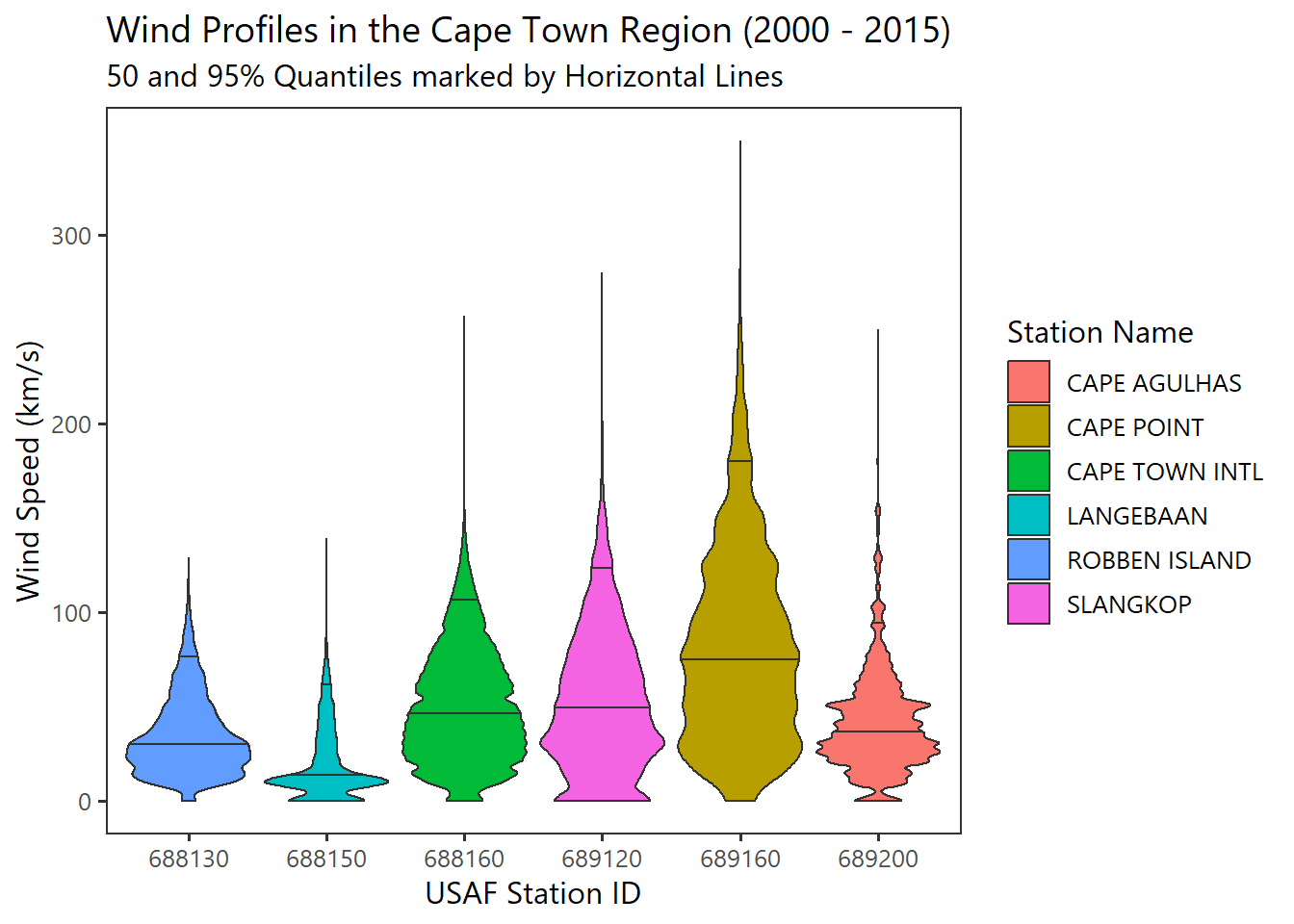
Here is a quick overview of the wind data distribution.

# quick plot of data
ggplot(Wind,aes(usaf_station, wind_speed, fill=location)) +
  geom_violin(scale="width",trim=TRUE,draw_quantiles = c(0.50,0.95)) + 
  xlab("USAF Station ID") + 
  ylab("Wind Speed (km/s)") + 
  labs(title="Wind Profiles in the Cape Town Region (2000 - 2015)",
                                   subtitle="50 and 95% Quantiles marked by Horizontal Lines",
       fill="Station Name") +
  theme_plain(base_size = 12)

Dan Gray

2017/11/19

Preparation of the Raw Data Files

Initial Cleaning

A First Look at the General Data Distribution