Territorial Expansion of Wolf Populations in Germany, 2000-2014

Summary

The reappearance and settlement of the grey wolf in eastern and northern Germany over the last 15 years has been a focal point of environmental discourse. Allowing passages of wilderness to bifurcate the land bolsters dwindling population numbers but increases the chances of contact with settlements and habitations.

Here I retrieved data to gain some personal insight into the spatial and temporal expansion of wolves over the last +/- 15 years.

Data Preparation

# load libraries
library(readr)
library(tidyverse)
library(DT)
library(deldir)

# load custom functions
source("static/data/ROAM.r")

# load locale data
wolf_data <- read_delim("static/data/wolves/wolf_data_2014.tsv",
                        "\t", escape_double = FALSE, trim_ws = TRUE)

One can include the implicit NAs for each year-location pair, and fill missing observations to build a “complete dataset”.

# complete the data by filling missing "data-slots"
complete.ts <-wolf_data %>% 
  complete(Jahr=full_seq(Jahr,1),nesting(Bundesland,Territorium),
           fill=list(Status="np",Repro="na",Welpen=0))

# make searchable table of complete data 
complete.ts %>% 
  datatable(., rownames = FALSE, filter="top",
            options = list(pageLength = 10, scrollX=F)) %>%
  DT::formatStyle(columns = c(1:6), fontSize = '85%')

One can create a lookup-table to hold the human-readable labels of the factors in the data.

# create annotations
labs_status <-data.frame(Status=c("e","p","r","np"),
                         Name=c("Single","Pair","Pack","Not Present"),
                         stringsAsFactors = FALSE)

Aggregating the Temporal Data

The wolves have aggregated in 2 main locations (as of 2014), namely Noctum and Neustadt.

# find unique locations with newborns
locations <- complete.ts %>% 
  group_by(Territorium) %>% 
  summarise(welpen_sum = sum(Welpen)) %>%
  arrange(desc(welpen_sum)) %>% filter(.,welpen_sum>0)

# most prevalent breeding locations
locations_select <- complete.ts %>% 
  group_by(Territorium) %>% 
  summarise(welpen_sum = sum(Welpen)) %>%
  arrange(desc(welpen_sum)) %>% filter(.,welpen_sum>10)

# quick plot 
locations_select %>% 
  ggplot(.,aes(fct_reorder(Territorium,welpen_sum,.desc = TRUE),welpen_sum)) + 
  geom_col() + 
  theme_plain(base_size = 10) + 
  scale_x_discrete(labels= abbreviate) +
  xlab("Territory") + ylab("Total Newborns (n)") +
  labs(title="Aggregated Count of Wolves in Eastern Germany, 2001-2014")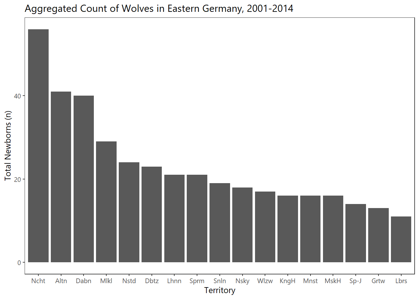

Spatial Distribution as a Proxy for Interaction Encounters

Spatial information (Lat/Lon) was manually retrieved using the www.latlon.net service.

# load coordinates information
coords_wolves <- read_delim("ststic/data/wolves/coords_wolves_2014.tsv","\t", 
                            escape_double = FALSE, trim_ws = TRUE)

# join with locale data
locations_mapped <-left_join(locations,coords_wolves)

One can quickly build up a figure which depicts the:

• aggregated total of newborns (+existing wolves) at any location
• draw this using an appropriate map projection (in this case AZ Equal Area)
• add the tessselation segments
• compute a 2d kernel density of the spatial distribution

A Voronoi Tesselation splits a plane into segments given by points ditributed within it so that each segment contains the point and the area which is closer to that point that any other

# compute voronoi tesselation
voronoi_gg <- deldir(locations_mapped$Lon,locations_mapped$Lat)

# build voronoi and density plot
ggplot(data=locations_mapped,aes(Lon,Lat)) +
  geom_segment(aes(x=x1,y=y1,xend=x2,yend=y2),
               size=0.5,color="grey",data=voronoi_gg$dirsgs) + 
  stat_density_2d(aes(fill = ..level..), 
                  geom = "polygon", alpha = 0.25, color = NA) +
  scale_fill_gradient2("Density", low = "white", mid = "yellow", high = "red", midpoint = 0.25) +
  geom_point(size=log(locations_mapped$welpen_sum)) +
  xlab("Longitude (degrees east)") + ylab("Latitude (degrees north)") + 
  labs(title="Wolf Prospensity in Eastern Germany",
       subtitle="With Voronoi Tesselations Marking Locales (AZ Equal Area Projection)") +  
  theme_plain(base_size = 11) + 
  coord_map("azequalarea",orientation = c(51.5,13,5)) +
    scale_y_continuous(limits=c(50,53),
                     breaks=c(50,51.5,53)) +
  scale_x_continuous(limits=c(8,16),
                     breaks=c(8,10,12,14,16))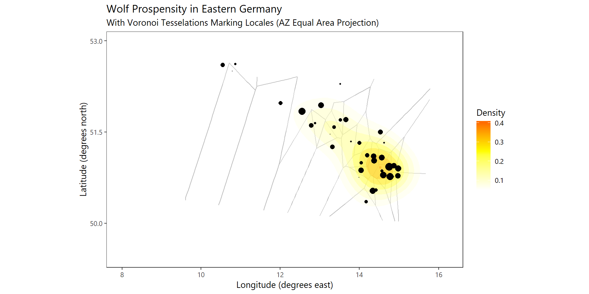

Plot an overview dashboard of population growth over time, in selected regions.

# select groups of interest
target_locales <- c("Sachsen", "Sachsen-Anhalt","Brandenburg", "Niedersachsen")
target_groups <- c("r","p")

stats <- complete.ts %>% 
  group_by(Jahr,Bundesland,Status) %>% 
  summarise(n=n()) %>% filter(., Status %in% target_groups) %>%
  filter(.,Bundesland %in% target_locales) %>% 
  left_join(labs_status)

# plot :: ts of groups over time per region
ggplot(stats,aes(Jahr,n)) + geom_point() + 
  geom_smooth(method="loess",se=FALSE) +
  facet_grid(Bundesland ~ Name) +
  theme_plain(base_size = 11) +
  xlab("Year") + ylab("Count") +
  scale_y_continuous(expand=c(0.1,0.1),
                     breaks=c(0,5,10)) +
  scale_x_continuous(expand=c(0.1,0.1),
                     breaks=c(2000,2004,2008,2012,2016))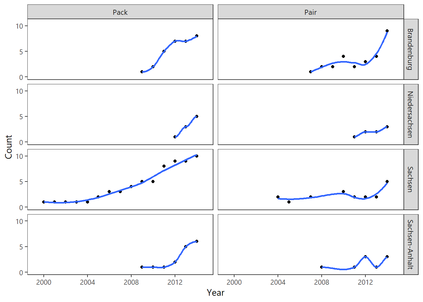

Build a complete map, with informative map layers, extra rasters and groupings.

library(leaflet)
library(leaflet.extras)

# work in progress :: testing heatmap functionality
leaflet(data = locations_mapped) %>% 
  addProviderTiles(providers$Esri.NatGeoWorldMap) %>%
  setView(12, 52, zoom = 6) %>% 
  addHeatmap(lng= ~Lon, lat = ~Lat, intensity = ~welpen_sum, blur = 20, radius = 15, max = 0.05) %>% 
  addCircleMarkers(~Lon,~Lat, stroke=FALSE, fillColor = "black",fillOpacity = 1, radius=2, popup = ~as.character(Territorium))