Summary
I’m fairly convinced that knowing something about the distribution of data is more important that the particular values that are within that distribution.
A mentor encouraged me to always inspect and understand the “wide-scale” patterns of the dataset before zomming in and becoming concerned with my particular question.
Here I use “ridge-plots” (density plots) to get a feeling for the overall dynamics of rainfall in Bremen over the modern observational record.
Initialise Packages
# load libraries
library(tidyverse)
library(forcats)
library(ggjoy)
library(ggridges)
library(viridis)
library(extrafont)
Prepare Monthly Data
# set up directories
setwd("C:/Users/daniel/Desktop/locstore/portfolio")
source("static/data/ROAM.r")
where <-getwd() # get home-dir

# load monthly data
monthly <-read_delim("static/data/gg_ridges/produkt_nieder_monat_18900101_20161231_00691.txt",";", escape_double = FALSE, trim_ws = TRUE)

# extract individual months and years
dateStr <-as.character(monthly$MESS_DATUM_BEGINN)
dateNum <-substr(dateStr, 1, 6) %>% as.double()
dateMonth <-substr(dateNum, 5, 6) %>% as.double()
dateYear <-substr(dateNum, 1, 4) %>% as.double()

# create temporary data.frame for modifications
frame <-mutate(monthly, frameID = dateNum-dateNum[1],
                month = dateMonth, year = dateYear)

# convert factors to numeric and fix NaN
frame$STATIONS_ID <-as.factor(frame$STATIONS_ID)
frame$monthFct <-as.factor(frame$month)
frame$MO_RR[frame$MO_RR==-999] <-NA
Seasonal Distribution
# select, mutate, and plot in one go
frame %>% select (MO_RR,monthFct,year) %>%
  mutate(labels=fct_recode(monthFct,"January" = "1", "February" = "2", "March" = "3",
                           "April" = "4","May"= "5", "June" = "6", "July" = "7",
                           "August" = "8", "September" = "9", "October" = "10",
                           "November" = "11", "December" = "12")) %>%
  ggplot(aes(x=MO_RR,y=labels %>% fct_rev())) +
  geom_density_ridges_gradient(aes(fill=labels)) +
  scale_fill_viridis(discrete=T,option="D", direction=-1,begin=.1,end=.9) +
  labs(x = "Total Precipitation (mm)", y = "Month of Year",
       title = "Distribution of Historical Monthly Rainfall in Bremen (1890-2015)",
       subtitle = "Data: Der Deutsche Wetter Dienst - Climate Data Center (CDC)") +
  theme_plain(base_size = 11) +
  theme(legend.position = "none")
## Picking joint bandwidth of 9.51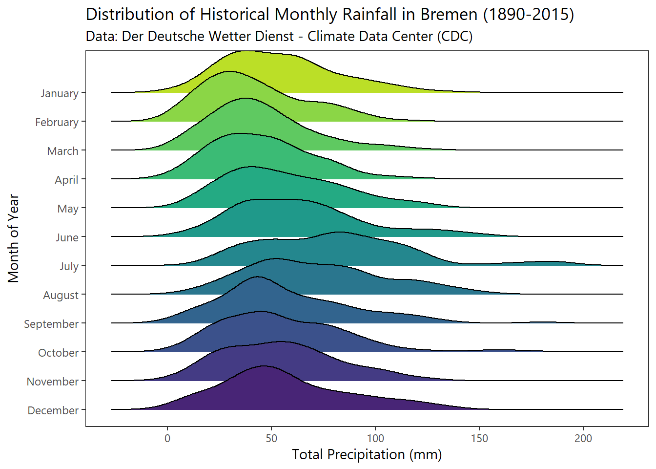
Historical Yearly Rainfall
# historical yearly totals
frame %>% filter(year<=2015 & year>=1891) %>%
  mutate(grp = cut(year, breaks = c(1890,1915,1940,1965,1990,2015),
                    labels=c("1891-1915","1916-1940","1941-1965","1966-1990","1991-2015"))) %>%
  select(MO_RR,monthFct,year,grp) %>%
  group_by(year,grp) %>%
  summarise(Total=sum(MO_RR)) %>% ungroup() %>%
  ggplot(aes(x=Total,y=grp %>% fct_rev(),fill=factor(..quantile..))) +
  stat_density_ridges(geom = "density_ridges_gradient",
                      calc_ecdf = TRUE, quantiles = c(0.025, 0.975)) +
  scale_fill_manual(name = "Probability", values = c("#FF0000A0", "#A0A0A0A0", "#0000FFA0"),
                    labels = c("(0, 0.025]", "(0.025, 0.975]", "(0.975, 1]")) +
  labs(x = "Total Precipitation (mm)", y = "Inteval",
       title = "Distribution of Historical Yearly Rainfall in Bremen (1891-2015)",
       subtitle = "Data: Der Deutsche Wetter Dienst - Climate Data Center (CDC)") +
  theme_plain(base_size = 11)
## Picking joint bandwidth of 42.6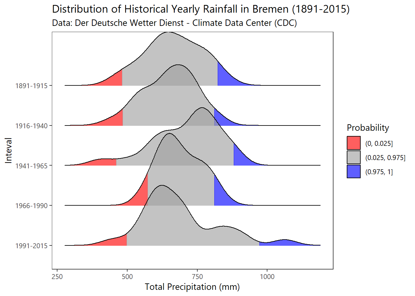
Peak Rainfall Month
# historical maximum peak rainfall month
frame %>% filter(year<=2015 & year>=1891) %>%
  mutate(grp = cut(year, breaks = c(1890,1915,1940,1965,1990,2015),
                   labels=c("1891-1915","1916-1940","1941-1965","1966-1990","1991-2015"))) %>%
  select(MO_RR,month,year,grp) %>%
  group_by(year,grp) %>% filter(MO_RR==max(MO_RR)) %>%
  ungroup() %>%
  ggplot(aes(x=month,y=grp %>% fct_rev()))+
  geom_density_ridges(aes(fill=grp),rel_min_height=0.01) +
  scale_fill_viridis(discrete=T,option="D", direction=-1,begin=.1,end=.9) +
  labs(x = "Month of Year", y = "Inteval",
       title = "Distribution of Historical Peak Rainfall Month in Bremen (1891-2015)",
       subtitle = "Data: Der Deutsche Wetter Dienst - Climate Data Center (CDC)") +
  theme_plain(base_size = 11) +
  theme(legend.position = "none")
## Picking joint bandwidth of 0.934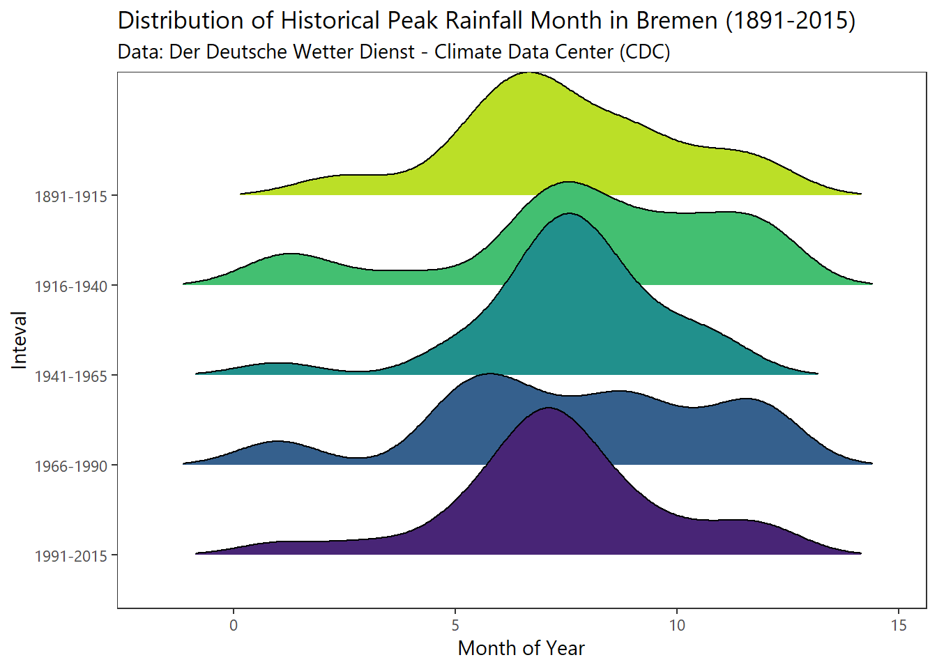
Prepare Daily Data
rm(dateMonth,dateNum,dateStr,dateYear,frame)

# set up directories
setwd("C:/Users/daniel/Desktop/locstore/portfolio")
where <-getwd() # get home-dir

# load daily data
daily <-read_delim("static/data/gg_ridges/produkt_nieder_tag_18900101_20161231_00691.txt",
                      ";", escape_double = FALSE, trim_ws = TRUE)
## Parsed with column specification:
## cols(
## STATIONS_ID = col_double(),
## MESS_DATUM = col_double(),
## QN_6 = col_double(),
## RS = col_double(),
## RSF = col_double(),
## SH_TAG = col_double(),
## eor = col_character()
## )# extract individual months and years
dateStr <-as.character(daily$MESS_DATUM)
dateNum <-substr(dateStr, 1, 6) %>% as.double()
dateMonth <-substr(dateNum, 5, 6) %>% as.double()
dateYear <-substr(dateNum, 1, 4) %>% as.double()
# create temporary data.frame for modifications
frame <-mutate(daily, frameID = dateNum-dateNum[1],
month = dateMonth, year = dateYear)
# convert factors to numeric and fix NaN
frame$STATIONS_ID <-as.factor(frame$STATIONS_ID)
frame$yearFct <-as.factor(frame$year)
frame$monthFct <-as.factor(frame$month)
frame$RS[frame$RS==-999] <-NAInspect Daily Data
# historical daily maximum within a month
frame_01 <-frame %>% filter(year<=2015 & year>=1891) %>%
mutate(grp = cut(year, breaks = c(1890,1915,1940,1965,1990,2015),
labels=c("1891-1915","1916-1940","1941-1965","1966-1990","1991-2015"))) %>%
select(RS,monthFct,yearFct,grp) %>%
group_by(monthFct,yearFct,grp) %>%
summarise(maxDay_Month=max(RS)) %>% ungroup()
# historical total within a month
frame_02 <-frame %>% filter(year<=2015 & year>=1891) %>%
mutate(grp = cut(year, breaks = c(1890,1915,1940,1965,1990,2015),
labels=c("1891-1915","1916-1940","1941-1965","1966-1990","1991-2015"))) %>%
select(RS,monthFct,yearFct,grp) %>%
group_by(monthFct,yearFct,grp) %>%
summarise(tot_Month=sum(RS)) %>% ungroup()
# lookup table :: join and summarise
frame_join <-frame_01 %>%
mutate(dayContMonth = (maxDay_Month/frame_02$tot_Month)*100) %>%
filter(dayContMonth>=50) %>% add_count(dayContMonth) %>%
group_by(grp) %>%
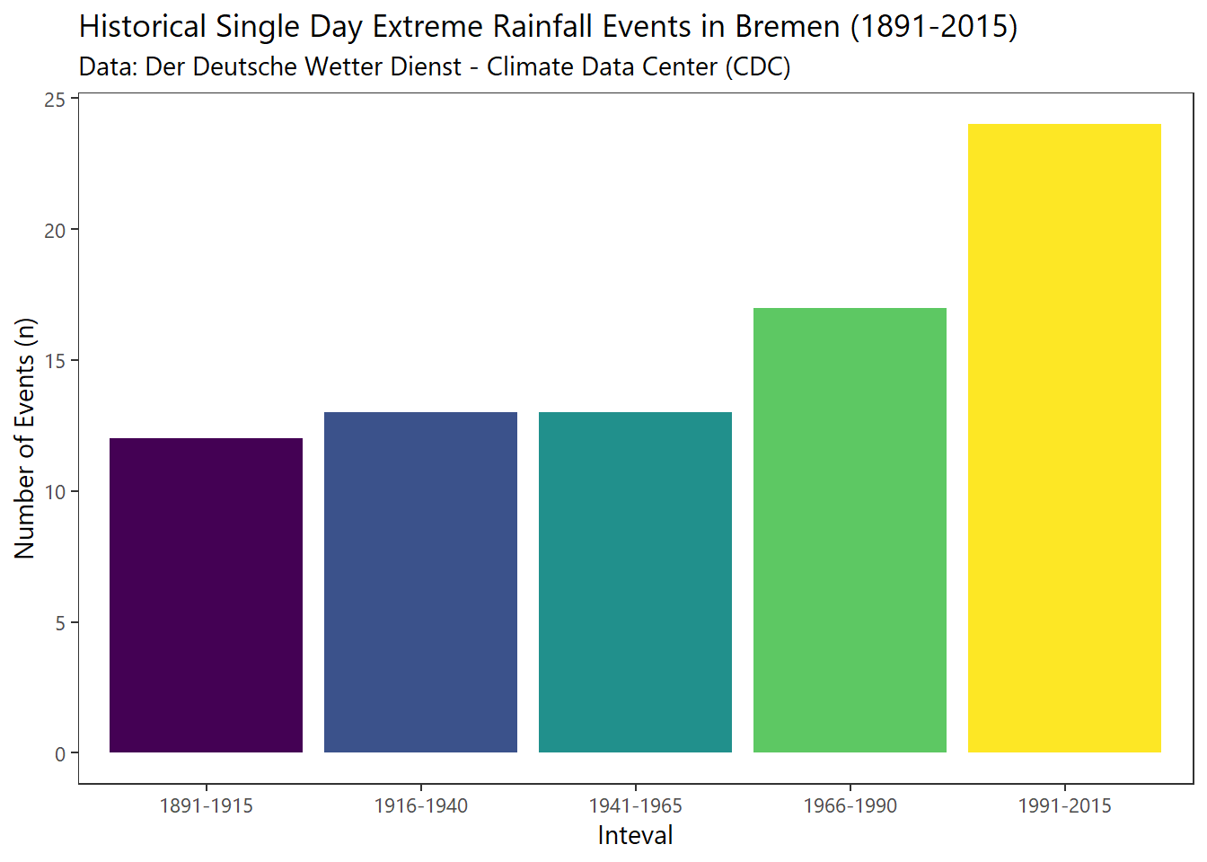
summarise(tots=sum(n))Doubling of “Single Day Downpours”
# plot N heavy rainfall "events" per interval
frame_join %>%
  ggplot() + geom_col(aes(x=grp,y=tots,fill=grp)) +
  scale_fill_viridis(discrete = T) +
  labs(x = "Inteval", y ="Number of Events (n)",
  title = "Historical Single Day Extreme Rainfall Events in Bremen (1891-2015)",
  subtitle = "Data: Der Deutsche Wetter Dienst - Climate Data Center (CDC)") +
  theme_plain(base_size = 11) +
  theme(legend.position = "none")