Summary
Bringing in standard binary files like Excel sheets into a relational datastore is a primary step in data-warehousing. From the store it can be queried at will by a variety of analytical interfaces and business intelligence suites.
Here I import records of National Footprint Accounts into a PostgreSQL table, which is then queried interactively from R for data exploration and visualization.
Implementation
We need to establish the connection to the PostgreSQL database, and provide the relevant username and password. To orientate oneself, one can use dbListTables to query all available tables.
# load libraries
library(tidyverse)
library(DBI)

# connect to database
con <- dbConnect(RPostgres::Postgres(),dbname="imports",
                 port=5432,user="USERNAME",password="PASSWORD")

# list all tables available
dbListTables(con)
We can query the table to infer the data-structure
# querying using postgreSQL syntax
query <- dbSendQuery(con, "SELECT *
                     FROM nfa LIMIT 10;")

dbFetch(query)
## country iso_code un_region un_subregion year record
## 1 Armenia ARM Asia Western Asia 1992 BiocapPerCap
## 2 Armenia ARM Asia Western Asia 1992 BiocapTotGHA
## 3 Armenia ARM Asia Western Asia 1992 EFConsPerCap
## 4 Armenia ARM Asia Western Asia 1992 EFConsTotGHA
## 5 Armenia ARM Asia Western Asia 1992 EFExportsPerCap
## 6 Armenia ARM Asia Western Asia 1992 EFExportsTotGHA
## 7 Armenia ARM Asia Western Asia 1992 EFImportsPerCap
## 8 Armenia ARM Asia Western Asia 1992 EFImportsTotGHA
## 9 Armenia ARM Asia Western Asia 1992 EFProdPerCap
## 10 Armenia ARM Asia Western Asia 1992 EFProdTotGHA
## crop_land grazing_land forest_land fishing_ground built_up_land
## 1 1.61129e-01 1.35023e-01 8.38355e-02 1.37180e-02 3.36685e-02
## 2 5.55813e+05 4.65763e+05 2.89191e+05 4.73202e+04 1.16140e+05
## 3 3.90923e-01 1.89137e-01 1.25000e-06 4.13764e-03 3.36685e-02
## 4 1.34849e+06 6.52429e+05 4.32784e+00 1.42728e+04 1.16140e+05
## 5 1.12491e-03 2.28304e-03 0.00000e+00 4.38381e-04 0.00000e+00
## 6 3.88038e+03 7.87533e+03 0.00000e+00 1.51220e+03 0.00000e+00
## 7 2.30919e-01 5.63969e-02 1.25000e-06 3.31238e-03 0.00000e+00
## 8 7.96555e+05 1.94541e+05 4.32784e+00 1.14261e+04 0.00000e+00
## 9 1.61129e-01 1.35023e-01 0.00000e+00 1.26364e-03 3.36685e-02
## 10 5.55813e+05 4.65763e+05 0.00000e+00 4.35894e+03 1.16140e+05
## carbon total percapita population
## 1 0.00000e+00 4.27374e-01 949.033 3.449
## 2 0.00000e+00 1.47423e+06 949.033 3.449
## 3 1.11223e+00 1.73009e+00 949.033 3.449
## 4 3.83662e+06 5.96795e+06 949.033 3.449
## 5 4.81904e-02 5.20368e-02 949.033 3.449
## 6 1.66233e+05 1.79501e+05 949.033 3.449
## 7 8.79112e-02 3.78541e-01 949.033 3.449
## 8 3.03250e+05 1.30578e+06 949.033 3.449
## 9 1.07250e+00 1.40359e+00 949.033 3.449
## 10 3.69960e+06 4.84168e+06 949.033 3.449dbClearResult(query)Compare ISO country-codes to country names.
query <-dbSendQuery(con,
        "SELECT DISTINCT(iso_code), country
        FROM nfa
        ORDER BY iso_code
        LIMIT 10;")

dbFetch(query)
## iso_code country
## 1 ABW Aruba
## 2 AFG Afghanistan
## 3 AGO Angola
## 4 ALB Albania
## 5 ARE United Arab Emirates
## 6 ARG Argentina
## 7 ARM Armenia
## 8 ATG Antigua and Barbuda
## 9 AUS Australia
## 10 AUT AustriadbClearResult(query)Determine the types of records (measurement-types) available.
query <-dbSendQuery(con,
        "SELECT DISTINCT(record)
        FROM nfa
        ORDER BY record;")

dbFetch(query)
## record
## 1 BiocapPerCap
## 2 BiocapTotGHA
## 3 EFConsPerCap
## 4 EFConsTotGHA
## 5 EFExportsPerCap
## 6 EFExportsTotGHA
## 7 EFImportsPerCap
## 8 EFImportsTotGHA
## 9 EFProdPerCap
## 10 EFProdTotGHAdbClearResult(query)The records are split into two broad types, those of the standard unit “global hectares” and those normalized to “per capita”. The resource capacity and utilization is split into 5 classes of activity
- Biocap: Biocapacity
- EFCons: Ecological Footprint of Consumption
- EFProd: Ecological Footprint of Production
A secondary hierarchy of measures towards exports or imports: - EFExports: Ecological Footprint towards Exports - EFImports: Ecological Footprint towards Imports
The relationship between Ecological Consumption and Ecological Production is related through the following formula:
EFConsumption = EFProduction + EFImports - EFExports
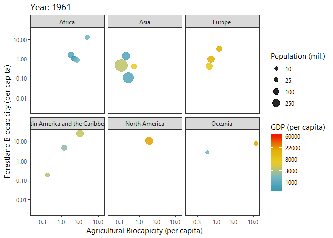
Investigating Biocapacities and Consumption Rates Globally
Below I query biocapicity records (per capita) for forestland and fishing grounds.
query <-dbSendQuery(con,
              "SELECT year,un_region, un_subregion,
              avg(forest_land) as forestland,
              avg(crop_land+grazing_land) as agricultural,
              sum(population) as tot_pop,
              avg(percapita) as percapita
              FROM nfa
              WHERE un_region != 'World'
              AND record = 'BiocapPerCap'
              GROUP BY year,un_region,un_subregion
              ORDER BY year,forestland DESC"
              )

growth_byYear <- dbFetch(query)
dbClearResult(query)
We can plot a ‘Hans Rosling’ like bubble-progression of the aggregated data using gganimate.
library(gganimate)
library(wesanderson)

pal <- wes_palette("Zissou1", 100, type = "continuous")

p<-ggplot(growth_byYear, aes(agricultural,forestland, size = tot_pop)) +
   geom_point(aes(colour=percapita),alpha=0.85) +
   scale_colour_gradientn(colours = pal,trans="log",
                          na.value = "transparent",
                          breaks=c(1000,3000,8000,22000,60000),
                          labels=c("1000","3000","8000","22000","60000"),
                          name="GDP (per capita)") +
   scale_y_log10() +
   scale_x_log10() +
   scale_size(range=c(2,12),breaks=c(10,25,100,250),
              name = "Population (mil.)") +
   facet_wrap(~un_region) +
   labs(title = 'Year: {frame_time}',
        x = 'Agricultural Biocapicity (per capita)',
        y = 'Forestland Biocapicity (per capita)') +
  theme_plain(base_size = 11) +
   transition_time(year) +
   ease_aes('linear')

animate(p, fps=6)