Summary
Moody blues or bubblegum-pop? It it possible to extract relevant metrics of positivity or negativity from song lyrics?
Here I again use the Billboard Hot 100 Year End Charts dataset to investigate which artists tend to produce music associated with positive or negative sentiment, based on lyrical content. I also briefly explore the temporal evolution of Chart Rankings based on overall sentiment.
Implementation
Setting up the spark environment requires a definition of how many cores, and RAM are accessible for processing.
library(sparklyr)
library(tidyverse)
library(tidytext)

# set up spark configuration
conf <- spark_config()
conf$`sparklyr.cores.local` <- 2
conf$`sparklyr.shell.driver-memory` <- "1G"
conf$spark.memory.fraction <- 0.7

# make connection
sc <- spark_connect(master="local",config = conf)

# read in data
billboard <- read.csv("C:/Users/eoedd/Desktop/locstore/portfolio/billboard_lyrics_1964-2015.csv",stringsAsFactors = FALSE)

# copy to spark
billboard <- copy_to(sc, billboard,overwrite=TRUE)
rm(billboard)


# list tables
src_tbls(sc)
## [1] "billboard"# create link to Spark Data Frame
hits <- tbl(sc, "billboard")For this local implementation, I choose to trim the data to a reasonable size for the ft_ operations. With a modern workstation the operation could be scaled for all the data.
The
ft_bucketizerfunction splits a variable into groups, in a similar way tocut(with some slight variations in the boundaries and inclusion constraints.)I choose to only complete cases of observations to avoid an error being thrown on the
ft_tokenizerstep. The functionft_tokenizertakes a string, converts it to lowercase and splits it by white-space.
At this point we need to collect the results to R for processing into a single word per row format.
The first step is packing the words into a list, as the type character. The individual words are then split into their own rows by unnesting from the list.
# subset data for testing
words_70s_80s <- hits %>%
  select(Artist,Year,Lyrics,Rank) %>%
  filter(Year > 1969 & Year < 1990) %>%
  na.omit() %>%
  filter(Rank < 51)

# group ranks
tiers <- c(0,11,21,31,41,51)
tier_labels <-c("1-10", "11-20", "21-30",
                   "31-40", "41-50")

# compute lyric-splits
lyrics_70s_80s <- words_70s_80s %>%
  ft_bucketizer("Rank","Tiers",splits=tiers) %>%
  ft_tokenizer("Lyrics","word") %>%
  collect() %>%
  mutate(word=lapply(word,as.character)) %>%
  unnest(word)
The sentiment scores are held in the tidytext packages.
# get sentiment matrix
sentiments <- get_sentiments("afinn")
glimpse(sentiments)
## Observations: 2,476
## Variables: 2
## $ word <chr> "abandon", "abandoned", "abandons", "abducted", "abducti...
## $ score <int> -2, -2, -2, -2, -2, -2, -3, -3, -3, -3, 2, 2, 1, -1, -1,...All that is left to do in terms of data preparation is inner-join the individuals lyrics to the sentiment scores. In this case I added a grouping variable to summarize the scores by Artist.
# calculate sentiments per artist
sent_artists <- lyrics_70s_80s %>%
  inner_join(sentiments,by="word") %>%
  group_by(Artist) %>%
  summarize(positivity=sum(score))

# most sentimental +ve
sent_artists %>%
  arrange(desc(positivity)) %>%
  top_n(15)
## # A tibble: 15 x 2
## Artist positivity
## <chr> <int>
## 1 kool the gang 427
## 2 whitney houston 418
## 3 jody watley 254
## 4 commodores 246
## 5 wings 201
## 6 billy idol 195
## 7 natalie cole 195
## 8 dr hook 191
## 9 stevie wonder 191
## 10 foreigner 172
## 11 donna summer 170
## 12 olivia newtonjohn 162
## 13 george michael 159
## 14 eagles 158
## 15 barbra streisand 157# least sentimental -ve
sent_artists %>%
arrange(positivity) %>%
top_n(-15)## # A tibble: 17 x 2
## Artist positivity
## <chr> <int>
## 1 bon jovi -75
## 2 duran duran -68
## 3 don mclean -57
## 4 kenny loggins -55
## 5 neil diamond -49
## 6 lou rawls -38
## 7 daryl hall john oates -37
## 8 eddie holman -37
## 9 the police -37
## 10 corey hart -36
## 11 klymaxx -36
## 12 bj thomas -35
## 13 john waite -35
## 14 pet shop boys -34
## 15 falco -33
## 16 juice newton -33
## 17 paper lace -33A few pleasant surprises here - just scrolling through the names in the respective “positive” and “negative” lists tends to evoke an association with feel-good (Kool & the Gang, Dr Hook) vs. reflective music (Neil Diamond, Falco). Naturally the samples are biased by occurrence. A better measure of artist sentimentality could be achieved by normalising by count (n).
An alternative inner-join gives us the most used lyrics and their associated sentiment.
# join tables
sentiment_lyrics <- lyrics_70s_80s %>%
  inner_join(sentiments,by="word")

# which words are used most
sentiment_lyrics %>%
  select(word,score) %>%
  group_by(score) %>%
  count(word,sort=TRUE) %>%
  arrange(desc(n)) %>%
  top_n(15)
## Selecting by n## # A tibble: 110 x 3
## # Groups: score [10]
## score word n
## <int> <chr> <int>
## 1 3 love 3138
## 2 -1 no 1261
## 3 2 like 1228
## 4 1 want 890
## 5 1 yeah 857
## 6 -2 ill 620
## 7 3 good 444
## 8 2 sweet 283
## 9 2 better 253
## 10 1 feeling 191
## # ... with 100 more rowsLastly its straightforward to trace the evolution of positivity or negativity in lyrics, split by ranking hierarchy over the period 1970-1989.
# compute score for average and total positivity
sent_ranks <- sentiment_lyrics %>%
  group_by(Year,Tiers) %>%
  summarize(tot_positivity=sum(score),
            avg_positivity=mean(score))

# plot of sentiment patterns
ggplot(sent_ranks,aes(Year,tot_positivity,colour=Tiers)) +
  geom_point() +
  geom_smooth(se=FALSE,method="loess") +
  ylab("Total Positivity Lyrical Content") +
  facet_wrap(~Tiers,nrow = 2) +
  theme_plain() + guides(colour=FALSE)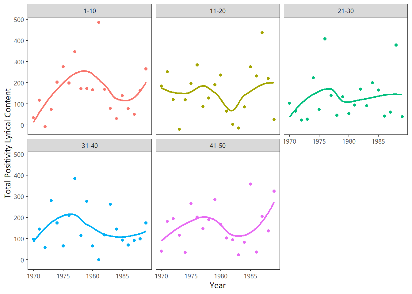
Interestingly the Top 10 songs have the most pronounced temporal variability (closely matched by those just making the Top 50) whereas intermediate rankings seems to have a more erratic emotional palette.
The early 1980’s seemed to be a time of rather negative sentiment. However 1981 was an outright anomaly for the most popular songs in that year!