Summary
Document (“NoSQL”) and relational (“SQL”) data-management systems are designed for two largely different scopes of work.
Document-based databases are built for flexibility, availability and bringing together ad-hoc data into a searchable environment.
Relational databases are implemented by stipulating the schema prior to data ingestion. They offer optimised querying on expensive hardware and are important mechanisms to establish a ‘universal truth’ within a business environment.
Here I compare the querying capabilities of these paradigms using two popular tools. This comparative analysis references the perspective of a BI-analyst i.e. ease of use, completeness, logic etc.
R is used as the core client: the packages mongolite and RPostgres are used as interfaces to call MongoDB and PostgreSQL 11 respectively.
Implementation
The nycflights2013 flights database is used for this exploration. It contains data of all flights departing from New York City in 2013 - including carrier, departure, delay and flight information.
library(mongolite)
library(tidyverse)
library(DBI)
First we establish the connections to each data-store.
# create new collection in MongoDB
con_mongo <- mongo(collection="delays",db="flights")

# connect to existing Postgre database
con_postgre <- dbConnect(RPostgres::Postgres(),dbname="postgres",
                 port=5432,user="USER",password="PASSWORD")
Followed by an import of the data where needed - in this case into MongoDB.
# import bson file into MongoDB
setwd("C:/Users/eoedd/Desktop/locstore/projects/mongodb/")
con_mongo$import(file("flights-dump.bson"),bson=TRUE)
## [1] 336776# list all tables available in Postgre database
dbListTables(con_postgre)## [1] "cities" "countries" "flights" "nfa"
## [5] "student_records" "weather"Some Basic Queries
# inspecting the collection contents
mongo_head <- con_mongo$find('{}',limit=5)
mongo_head
## year month day dep_time dep_delay arr_time arr_delay carrier tailnum
## 1 2013 1 1 517 2 830 11 UA N14228
## 2 2013 1 1 533 4 850 20 UA N24211
## 3 2013 1 1 542 2 923 33 AA N619AA
## 4 2013 1 1 544 -1 1004 -18 B6 N804JB
## 5 2013 1 1 554 -6 812 -25 DL N668DN
## flight origin dest air_time distance hour minute
## 1 1545 EWR IAH 227 1400 5 17
## 2 1714 LGA IAH 227 1416 5 33
## 3 1141 JFK MIA 160 1089 5 42
## 4 725 JFK BQN 183 1576 5 44
## 5 461 LGA ATL 116 762 5 54# inspecting using postgreSQL syntax
postgre_head <- dbSendQuery(con_postgre, "SELECT *
FROM flights LIMIT 5;
")Specifying and filtering down to specific fields:values / rows.
# retrieving a basic 'subset' using MongoDB
mongo_sub <- con_mongo$find('{"carrier" : "UA", "month" : 1, "day" : 1, "origin" : "JFK"}')
mongo_sub
## year month day dep_time dep_delay arr_time arr_delay carrier tailnum
## 1 2013 1 1 558 -2 924 7 UA N29129
## 2 2013 1 1 611 11 945 14 UA N532UA
## 3 2013 1 1 803 3 1132 -12 UA N510UA
## 4 2013 1 1 829 -1 1152 -8 UA N554UA
## 5 2013 1 1 1112 12 1440 2 UA N517UA
## 6 2013 1 1 1127 -3 1504 16 UA N518UA
## 7 2013 1 1 1422 -3 1748 -11 UA N502UA
## 8 2013 1 1 1522 -8 1858 3 UA N512UA
## 9 2013 1 1 1726 -3 2042 -18 UA N557UA
## 10 2013 1 1 1750 0 2109 -6 UA N525UA
## 11 2013 1 1 1840 -5 2223 -3 UA N508UA
## flight origin dest air_time distance hour minute
## 1 194 JFK LAX 345 2475 5 58
## 2 303 JFK SFO 366 2586 6 11
## 3 223 JFK SFO 369 2586 8 3
## 4 443 JFK LAX 360 2475 8 29
## 5 285 JFK SFO 364 2586 11 12
## 6 703 JFK LAX 357 2475 11 27
## 7 257 JFK SFO 362 2586 14 22
## 8 530 JFK LAX 356 2475 15 22
## 9 512 JFK SFO 347 2586 17 26
## 10 535 JFK LAX 345 2475 17 50
## 11 389 JFK SFO 357 2586 18 40# retrieving a subset using Postrgre
postgre_sub <- dbSendQuery(con_postgre, "SELECT *
FROM FLIGHTS
WHERE CARRIER = 'UA' AND
MONTH_ = 1 AND
DAY_ = 1 AND
ORIGIN = 'JFK';
")Custom Queries
Using mongolite one can specific a more complex query, by using the following arguments:
sortto return the data sorted on a particular fieldfieldsspecifies the desired fields to be returnedlimitoptionally restricts the number of returned documents
# specifying which columns to return with sort, fields and limit
mongo_custom <- con_mongo$find('{"carrier" : "DL", "month" : 12, "day" : 24}',
                       sort = '{"dep_delay" : -1}',
                       fields = '{"tailnum" : true, "flight" : true,
                       "origin" : true, "dest" : true, "dep_delay" : true}',
                       limit = 10)

mongo_custom
## _id dep_delay tailnum flight origin dest
## 1 5c921ec275741c1cb41d279a 142 N976DL 2113 LGA TPA
## 2 5c921ec275741c1cb41d28ff 135 N976DL 1935 LGA TPA
## 3 5c921ec275741c1cb41d27e8 66 N3737C 457 JFK SLC
## 4 5c921ec275741c1cb41d27f9 45 N994AT 1567 EWR ATL
## 5 5c921ec275741c1cb41d27f5 42 N900DE 2552 LGA SRQ
## 6 5c921ec275741c1cb41d274a 37 N319NB 2119 LGA MSP
## 7 5c921ec275741c1cb41d28be 37 N950DL 456 JFK DTW
## 8 5c921ec275741c1cb41d289f 29 N187DN 417 JFK LAX
## 9 5c921ec275741c1cb41d2730 25 N969DL 2442 JFK FLL
## 10 5c921ec275741c1cb41d288b 20 N376DA 2043 JFK SJU# specifying columns to return using WHERE, ORDER BY and LIMIT
postgre_custom <- dbSendQuery(con_postgre,"SELECT
tailnum, flight, origin, dest, dep_delay
FROM flights
WHERE carrier = 'DL' AND
month_ = 12 AND
day_ = 24
ORDER BY dep_delay DESC
LIMIT 10;
")Optimizing Query Performance
To speed up MongoDB queries one can add a set of indices on a particular field(s), which will be queried often. This is particular recommended for large and complex stores.
We can use the microbenchmark package to compare the efficiency improvements across the various implementations.
library(microbenchmark)

mon_no_ind <- microbenchmark("Mongo_No_Index" = {
  con_mongo$find('{}', sort = '{"dep_delay" : -1 }',
                           limit=50000)
  },
  times=10
)
The indexed fields are created using $index and add.
con_mongo$index(add = '{"dep_delay" : -1}')## v key._id key.dep_delay name ns
## 1 2 1 NA _id_ flights.delays
## 2 2 NA -1 dep_delay_-1 flights.delaysmon_ind <- microbenchmark("Mongo_Index" = {
con_mongo$find('{}', sort = '{"dep_delay" : -1 }',
limit=50000)
},
times=10
)
# remove indexing on field
con_mongo$index(remove = "dep_delay_-1")## v _id name ns
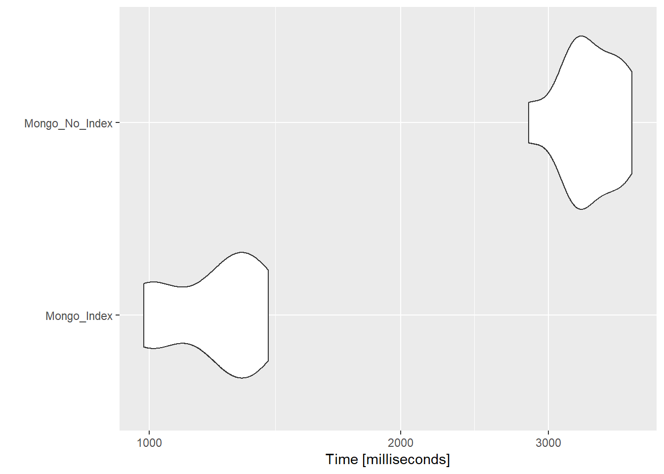
## 1 2 1 _id_ flights.delaysUsing ggplot2 we can autoplot the combined results. Indexing brings a 3X speed increase for this particular query.
mon_results<-rbind(mon_ind,mon_no_ind)
autoplot(mon_results)
The same approach can be used in PostgreSQL tables using INDEXES.
# querying without an index
pos_no_ind <- microbenchmark("Postgre_No_Index" = {
  postgre_no_index_find <- dbSendQuery(con_postgre, " SELECT *
                                  FROM flights
                                  ORDER BY dep_delay
                                  LIMIT 50000
                                  ")
 dbFetch(postgre_no_index_find)
 },
 times=10
)
One uses the CREATE INDEX command to add an index ON a given column within a table.
# querying with an index
postgre_index <- dbSendQuery(con_postgre,"CREATE INDEX
                              dep_index ON flights (dep_delay)
                              ")

pos_ind <- microbenchmark("Postgre_Index" = {
  postgre_index_find <- dbSendQuery(con_postgre, " SELECT *
                                  FROM flights
                                  ORDER BY dep_delay
                                  LIMIT 50000
                                  ")
 dbFetch(postgre_index_find)
 },
 times=10
)

# drop the index created
postgre_drop_index <- dbSendQuery(con_postgre,"DROP INDEX
                              dep_index
                              ")
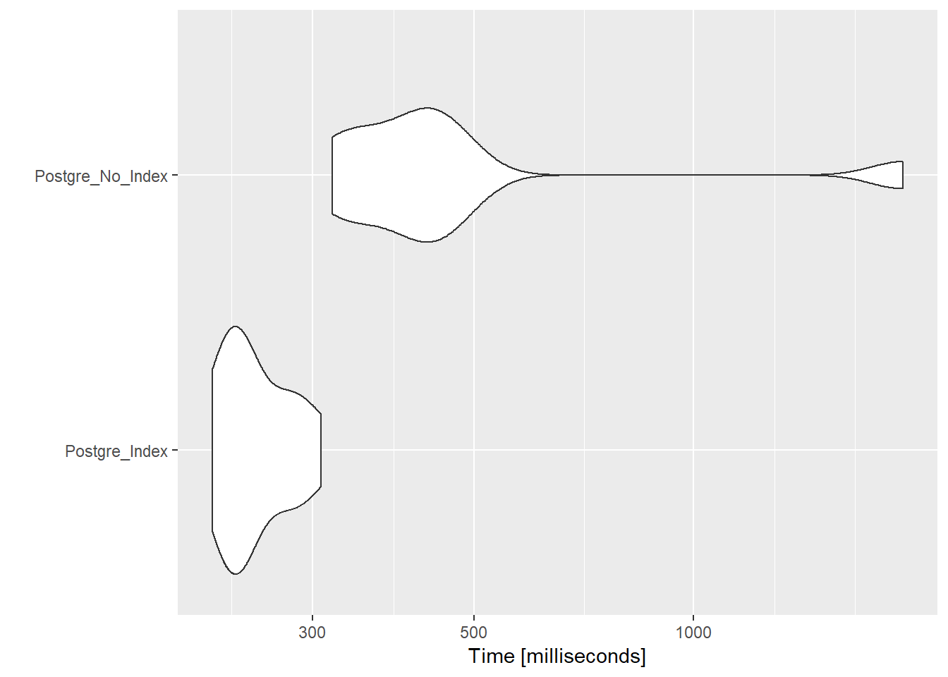
Indexing in this case brings again an ~3X speed increase. Its also worth noting PostgreSQL performs about 3X faster on these set of queries than MongoDB. I can imagine using more complex queries will even out the performance discrepancy.
pos_results<-rbind(pos_ind,pos_no_ind)
autoplot(pos_results)
To clean up the MongoDB environment we can drop associated collections using the $drop command.
In an upcoming post I will look at the great aggregation and graph-lookup features MongoDB offers.
# drop a given collection
con_mongo$drop()

# count collections
con_mongo$count()
## [1] 0# retrieve information about the connection
con_mongo$info()## List of 4
## $ collection: chr "delays"
## $ db : NULL
## $ stats : NULL
## $ server :List of 28
## ..$ host : chr "DESKTOP-55H3A25"
## ..$ version : chr "4.0.11"
## ..$ process : chr "C:\\Program Files\\MongoDB\\Server\\4.0\\bin\\mongod.exe"
## ..$ pid : num 5904
## ..$ uptime : num 344199
## ..$ uptimeMillis : num 3.44e+08
## ..$ uptimeEstimate : num 344198
## ..$ localTime : POSIXct[1:1], format: "2019-08-23 21:41:40"
## ..$ asserts :List of 5
## ..$ connections :List of 4
## ..$ encryptionAtRest :List of 1
## ..$ extra_info :List of 6
## ..$ globalLock :List of 3
## ..$ locks :List of 3
## ..$ logicalSessionRecordCache:List of 11
## ..$ network :List of 7
## ..$ opLatencies :List of 4
## ..$ opReadConcernCounters :List of 6
## ..$ opcounters :List of 6
## ..$ opcountersRepl :List of 6
## ..$ storageEngine :List of 5
## ..$ tcmalloc :List of 2
## ..$ transactions :List of 9
## ..$ transportSecurity :List of 5
## ..$ wiredTiger :List of 18
## ..$ mem :List of 6
## ..$ metrics :List of 11
## ..$ ok : num 1